Disclaimer: The opinions expressed in this article are my own and do not represent the views of Google. This content is based solely on publicly available information.
This article is Part 7 of the series, but you do not need Parts 1-6 — basic PyTorch familiarity and the idea that a Transformer predicts one token at a time is enough.
TL;DR of Parts 1-6. We have built every component of a Transformer from scratch in PyTorch: word embeddings (Part 1), RNN/LSTM as a sequential precursor (Part 2), scaled dot-product attention (Part 3), multi-head attention with positional encoding (Part 4), the Encoder Layer with residuals + LayerNorm + FFN (Part 5), and the Decoder Layer with masked self-attention + cross-attention to assemble the full architecture (Part 6). That gave us every parameter we want, none we do not. Now we shift to how the field actually works in 2026: download a pre-trained Transformer that someone with serious compute already trained, and use it. Part 6 covered the Decoder & Full Transformer architecture we just finished.
Series navigation
| Part | Topic |
|---|---|
| 1 | Introduction & Word Embeddings |
| 2 | From RNNs to LSTMs |
| 3 | The Attention Mechanism |
| 4 | Multi-Head Attention & Positional Encoding |
| 5 | The Transformer Encoder |
| 6 | The Decoder & Full Transformer |
| 7 (this article) | Pre-trained Models & Tokenization |
| 8 | Supervised Fine-Tuning |
| 9 | LoRA & QLoRA |
| 10 | DPO Alignment |
Parts 1–6 built every component of the Transformer from scratch: embeddings, attention, the encoder, and the decoder. That gave us a complete mental model but nothing pre-trained — every weight was random. In this part we make the shift that every real ML practitioner makes: instead of training from scratch, we download a pre-trained LLM from the Hugging Face Hub and start using it immediately. Along the way we look closely at the sub-word tokenizer that bridges raw text and integer IDs, generate text with both greedy and sampling decoding, and see why instruction-tuned models require a specific chat template to behave as intended.
A pre-trained model in two lines of code
The most immediate benefit of the Hugging Face ecosystem is that loading any of the thousands of models on the Hub requires almost no code. Before looking at tokenization or generation, let us verify that loading actually works and confirm we have a real, non-trivial model.
The transformers library is to LLMs what torchvision is to image models — a unified interface to thousands of pre-trained checkpoints. Loading one is two lines:
from transformers import AutoModelForCausalLM, AutoTokenizer

MODEL = "Qwen/Qwen2.5-0.5B-Instruct"
tokenizer = AutoTokenizer.from_pretrained(MODEL)
model     = AutoModelForCausalLM.from_pretrained(MODEL, torch_dtype="auto")

print(f"Model  : {MODEL}")
print(f"Params : {sum(p.numel() for p in model.parameters()) / 1e6:.1f}M")
print(f"Vocab  : {tokenizer.vocab_size:,}")
Output:
Model  : Qwen/Qwen2.5-0.5B-Instruct
Params : 494.0M
Vocab  : 151,936
Behind those two lines: download ~1 GB of weights from the Hub, parse the safetensors (memory-mapped tensor file format, faster + safer than pickle-based .bin) files, instantiate the right architecture (Qwen2 in this case), and load every parameter. The first call caches everything locally so subsequent runs are instant.
Why Qwen2.5-0.5B? It is a real instruction-tuned (post-trained on (prompt, answer) pairs to follow instructions) LLM (released by Alibaba in late 2024) (Qwen2.5 family released September 2024; see the Alibaba/Qwen2.5 technical report.) but small enough — ~494M (marketed as 0.5B) parameters — to fit comfortably on a CPU-only laptop and even sit inside a Kaggle T4 GPU’s VRAM with room to fine-tune. The same code runs unchanged on Llama-3-8B, Mistral-7B, or any other open-weights causal LM.
AutoModelForCausalLM is a factory that inspects the model config and returns the right architecture. “CausalLM” means the model predicts the next token given all previous tokens — exactly the autoregressive generation pattern we built in Part 6, scaled up about ten thousand times.
Tokenization is not what you think
With the model loaded, the next question is: how does raw text actually become the integer IDs the model expects? Throughout Parts 1–6 we implicitly assumed a simple word-to-index mapping. Real tokenizers are significantly more sophisticated, and understanding them changes how you think about prompt length, multilingual performance, and vocabulary size trade-offs.
The simple version is “split on whitespace and look up each word in a vocabulary”. The real version is far more interesting.
Modern LLMs use sub-word tokenization — typically Byte-Pair Encoding (BPE) or its WordPiece / SentencePiece variants. The tokenizer is itself trained on a large corpus to find the most useful sub-word units.
How BPE works
BPE starts with a character-level vocabulary and iteratively merges the most frequent adjacent pair into a new token:
Iteration 0: vocabulary = {"l","o","w","e","r","n","s","t","i","g","h",...}
Corpus:       "l o w" "l o w e r" "n e w e s t" "w i d e s t" ...

Most frequent pair: ("e", "s") → merge into "es"
Most frequent pair: ("es", "t") → merge into "est"
Most frequent pair: ("l", "o") → merge into "lo"
Most frequent pair: ("lo", "w") → merge into "low"
...
After 50,000 merge operations (the typical setting for GPT-2), common words like "the", "and", "computer" get a single token each. Rare or compound words get split into pieces. Words from any language can be encoded by falling back to character (or even byte) level pieces.
The vocabulary size choices used in practice:
- GPT-2: 50,257 tokens
- GPT-3/4: 100,277 tokens
- Llama 3: 128,256 tokens
- Qwen2.5: 151,936 tokens
Larger vocabularies mean fewer tokens per sentence (more efficient computation) but larger embedding tables.
Tokenization in action
I tokenized four sentences with the GPT-2 tokenizer (real BPE, captured from an actual call to tokenizer.encode):
from transformers import AutoTokenizer

tok = AutoTokenizer.from_pretrained("gpt2")

sentences = [
    "Hello, world!",
    "The Transformer is a neural network.",
    "Olá, mundo! Tudo bem?",
    "obrigado pela sua atenção.",
]

for s in sentences:
    ids  = tok.encode(s)
    toks = tok.convert_ids_to_tokens(ids)
    print(f"Text   : {s}")
    print(f"Tokens : {toks}")
    print(f"IDs    : {ids}")
    print()
Output:
Text   : Hello, world!
Tokens : ['Hello', ',', 'Ġworld', '!']
IDs    : [15496, 11, 995, 0]

Text   : The Transformer is a neural network.
Tokens : ['The', 'ĠTrans', 'former', 'Ġis', 'Ġa', 'Ġneural', 'Ġnetwork', '.']
IDs    : [464, 3602, 16354, 318, 257, 17019, 3127, 13]

Text   : Olá, mundo! Tudo bem?
Tokens : ['Ol', 'á', ',', 'Ġmund', 'o', '!', 'ĠT', 'udo', 'Ġbe', 'm', '?']
IDs    : [30098, 6557, 11, 27943, 78, 0, 309, 12003, 307, 76, 30]

Text   : obrigado pela sua atenção.
Tokens : ['ob', 'rig', 'ado', 'Ġp', 'ela', 'Ġsu', 'a', 'Ġat', 'en', 'ç', 'ão', '.']
IDs    : [672, 4359, 4533, 279, 10304, 424, 64, 379, 268, 16175, 28749, 13]
Several useful observations jump out:
- The leading
Ġmarker indicates a token that includes a leading space.'ĠTrans'is ” Trans”, not “Trans”. This lets BPE handle the difference between word-internal and word-initial occurrences correctly. - Common words get one token, rare ones get split.
'Hello'is a single token (id 15496).'Transformer'becomes two:'ĠTrans' + 'former'. - Non-English text gets split aggressively.
'mundo'(Portuguese for “world”) is two tokens['Ġmund', 'o'].'atenção'is six tokens because the GPT-2 BPE was trained almost exclusively on English. - No
[UNK]token ever. BPE can encode anything by falling back to character (or even byte) level. The vocabulary is exhaustive.
For the same four sentences, here are the token counts compared between word-level (whitespace split) and the GPT-2 BPE tokenizer:
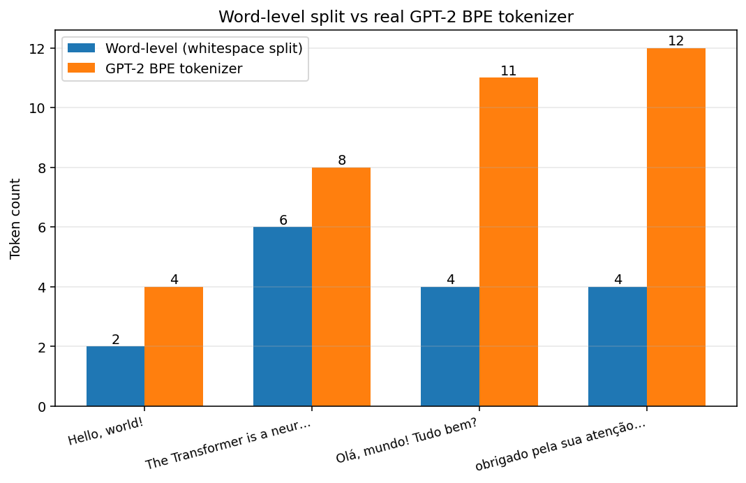
Figure 1: Word-level split vs real GPT-2 BPE tokenizer token counts for four sentences. (‘Words’ here = len(sentence.split()); punctuation is fused to adjacent tokens by whitespace splitting.)
For English, the counts are similar (2 vs 4 for “Hello, world!”; 6 vs 8 for the Transformer sentence). For Portuguese, the gap widens dramatically: 4 words become 11–12 BPE tokens because GPT-2’s tokenizer was trained almost exclusively on English and falls back to splitting unfamiliar words into smaller pieces. The practical consequence is that processing a Portuguese conversation costs roughly 2× the inference of an equivalent English one. Dedicated multilingual tokenizers (Llama-3, Qwen2.5) fix this by training BPE on multilingual corpora.
Generating text — greedy vs sampling
With tokenization understood, we can now close the loop: encode a prompt to IDs, run the model, and decode the generated IDs back to text. The two most common decoding strategies — greedy and sampling — produce very different behaviours, and knowing when to use each is a practical necessity.
Once we have a model and a tokenizer, generation is one method call:
import torch
from transformers import AutoModelForCausalLM, AutoTokenizer

MODEL = "Qwen/Qwen2.5-0.5B-Instruct"
tokenizer = AutoTokenizer.from_pretrained(MODEL)
model     = AutoModelForCausalLM.from_pretrained(MODEL)

prompt = "The key idea behind the Transformer architecture is"
inputs = tokenizer(prompt, return_tensors="pt")

with torch.no_grad():
    outputs = model.generate(
        **inputs,
        max_new_tokens=80,
        do_sample=False,                # greedy decoding
        pad_token_id=tokenizer.eos_token_id,
    )

generated = tokenizer.decode(outputs[0], skip_special_tokens=True)
print(generated)
Output:
The key idea behind the Transformer architecture is self-attention, which allows
each element in a sequence to attend to all other elements. This is different from
recurrent neural networks (RNNs), which process sequences sequentially. Self-attention
is computationally efficient and can be parallelized, making Transformers well-suited
for large-scale tasks like language modeling.
do_sample=False is greedy decoding: at every step, pick the single most probable next token. Because it is deterministic, the same prompt always produces the same output.
For more variety, we sample from the softmax distribution instead:
import torch
from transformers import AutoModelForCausalLM, AutoTokenizer

MODEL = "Qwen/Qwen2.5-0.5B-Instruct"
tokenizer = AutoTokenizer.from_pretrained(MODEL)
model     = AutoModelForCausalLM.from_pretrained(MODEL)

prompt = "The key idea behind the Transformer architecture is"
inputs = tokenizer(prompt, return_tensors="pt")

torch.manual_seed(42)
with torch.no_grad():
    outputs = model.generate(
        **inputs,
        max_new_tokens=80,
        do_sample=True,
        temperature=0.7,       # <1 → sharper distribution (less random)
        top_p=0.9,             # nucleus: keep top tokens summing to 90% probability
        pad_token_id=tokenizer.eos_token_id,
    )
print(tokenizer.decode(outputs[0], skip_special_tokens=True))
Output (Apple M4 Mac mini, 16 GB unified memory, macOS; python==3.9, transformers==4.57.6, torch==2.8.0; CPU inference):
The key idea behind the Transformer architecture is to learn representations of input data by mapping it into a higher-dimensional space, where each dimension captures different features. This leads to an increase in computational efficiency and parallelism compared to traditional convolutional neural networks (CNNs). However, this method can be challenging to implement efficiently due to the need for large memory resources.

To address this challenge, researchers have proposed various ways to reduce the size of the intermediate
To reproduce locally:
pip install "transformers>=4.57" "torch>=2.8". Both wheels are arm64-native on Apple Silicon — no extra flags needed.- Save the snippet above as
qwen_sampling.pyandpython3 qwen_sampling.py. - First run downloads
Qwen/Qwen2.5-0.5B-Instruct(~1 GB of fp32 weights) into~/.cache/huggingface/hub/; subsequent runs reuse the cache. - End-to-end generation took single-digit seconds on a modern laptop CPU; roughly 2-5× faster on Apple Silicon GPU via MPS (Apple’s Metal Performance Shaders backend) at this model size. The 0.5B model uses ~2 GB of resident memory in fp32 — fits comfortably alongside a browser and IDE. For Apple Silicon GPU acceleration, append
.to("mps")to bothmodelandinputs. - Output is deterministic given
torch.manual_seed(42)and identical library versions. Different transformers/torch minor versions can shift the sample because of changes totop_pfiltering tie-breaks.
temperature divides the logits (pre-softmax scores per vocabulary token) before softmax:
temperature=1.0: unchanged distributiontemperature=0.7: more concentrated, higher-probability tokens preferredtemperature=1.5: more spread out, more creative but also more likely to generate gibberish
top_p=0.9 (nucleus sampling — sample from the smallest token set whose cumulative probability exceeds p): at each step, keep the smallest set of tokens whose cumulative probability is at least 0.9, then renormalize and sample. This prunes the long tail of unlikely tokens.
import torch
import torch.nn.functional as F

# Hypothetical logits for 5 tokens
logits = torch.tensor([3.0, 2.0, 1.5, 0.5, 0.2])

for temp in [0.5, 1.0, 2.0]:
    probs = F.softmax(logits / temp, dim=0)
    print(f"Temp {temp}: {[round(p, 3) for p in probs.tolist()]}")
Output:
Temp 0.5: [0.836, 0.113, 0.042, 0.006, 0.003]
Temp 1.0: [0.577, 0.212, 0.129, 0.047, 0.035]
Temp 2.0: [0.383, 0.232, 0.181, 0.11, 0.094]
Lower temperature concentrates probability on the top token (0.836 at temp=0.5 vs 0.383 at temp=2.0). Higher temperature flattens the distribution, introducing more variety.
Chat templates
Generation with a raw text prompt works, but instruction-tuned models were fine-tuned on structured conversations, not raw continuations. Feeding them plain text produces noticeably worse outputs — you have to speak their language, which means using the chat template the model was trained on.
There is one last detail that trips up most newcomers. The model we loaded — Qwen/Qwen2.5-0.5B-Instruct — was fine-tuned to follow instructions. It expects input in a very specific format with special delimiter tokens marking who is talking:
<|im_start|>system
You are a helpful assistant.<|im_end|>
<|im_start|>user
Your question here<|im_end|>
<|im_start|>assistant
If you just feed it raw text, you will get back the model’s “complete this document” behaviour — which is far less helpful than the conversational mode it was trained for. To get the right behaviour, you build a list of message dicts and call apply_chat_template:
from transformers import AutoModelForCausalLM, AutoTokenizer
import torch

MODEL = "Qwen/Qwen2.5-0.5B-Instruct"
tokenizer = AutoTokenizer.from_pretrained(MODEL)
model     = AutoModelForCausalLM.from_pretrained(MODEL)

messages = [
    {"role": "system", "content": "You are a helpful AI tutor."},
    {"role": "user",   "content": "In one sentence, what is self-attention?"},
]

input_ids = tokenizer.apply_chat_template(
    messages,
    return_tensors="pt",
    add_generation_prompt=True,    # appends "<|im_start|>assistant\n"
)

with torch.no_grad():
    output_ids = model.generate(
        input_ids,
        max_new_tokens=60,
        do_sample=False,
        pad_token_id=tokenizer.eos_token_id,
    )

# Decode only the generated part (skip the input tokens)
new_tokens = output_ids[0, input_ids.shape[1]:]
print(tokenizer.decode(new_tokens, skip_special_tokens=True))
Output:
Self-attention is a mechanism that allows each token in a sequence to compute
its representation by attending to all other tokens in the same sequence,
weighted by their relevance.
apply_chat_template knows the model’s specific format and renders the messages into the right structured string before tokenizing. Every chat-tuned model on the Hub ships its own template, so the same code works across Llama, Qwen, Gemma, Mistral, Phi, etc.
Chat template formats differ by model
| Model family | Format style |
|---|---|
| Qwen2.5 | <|im_start|>role\n...<|im_end|> |
| Llama-3 | <|begin_of_text|>...<|start_header_id|>role<|end_header_id|>... |
| Gemma | <start_of_turn>role\n...<end_of_turn> |
| Mistral | [INST] user [/INST] assistant </s> |
Always use apply_chat_template rather than manually constructing these strings — the templates handle edge cases (system prompts that some models do not support, multi-turn spacing, etc.) that are easy to get wrong.
Model sizes and hardware requirements
Before you can run any of the models in the table above, you need to know whether your hardware can hold them. Understanding the memory math up front saves hours of failed runs and out-of-memory errors.
Knowing how much VRAM a model needs before you try to load it prevents the most common beginner frustration. The rule of thumb: 1B parameters in fp16/bf16/fp32 (16-bit IEEE, 16-bit brain-float, 32-bit float) — 1B in fp16 requires approximately 2 GB of GPU memory just to store the weights.
VRAM ≈ params × dtype_bytes + KV_cache (stored key/value projections from previous tokens, reused on each decode step)(batch, ctx_len, n_layers, hidden_dim); the table assumes batch=1 and dtype as labelled.
| Model | Parameters | fp16 weights | fp16 + KV cache (4K ctx) | Minimum GPU |
|---|---|---|---|---|
| Qwen2.5-0.5B | 494M | ~1 GB | ~1.5 GB | GTX 1070 (8 GB) |
| Qwen2.5-1.5B | 1.5B | ~3 GB | ~4 GB | RTX 3060 (12 GB) |
| Qwen2.5-7B | 7.6B | ~15 GB | ~18 GB | RTX 3090 (24 GB) |
| Llama-3-8B | 8B | ~16 GB | ~20 GB | RTX 4090 (24 GB) |
| Llama-3-70B | 70B | ~140 GB | 160+ GB | 2× A100 (160 GB) |
For inference-only (not training), quantization compresses these significantly. A 7B model in INT4 fits in ~5 GB of VRAM — single-GPU inference on a gaming card.
device_map="auto" is the simplest way to handle multi-GPU or CPU-offload situations:
from transformers import AutoModelForCausalLM

# Automatically spread across available GPUs, then RAM, then disk if needed
model = AutoModelForCausalLM.from_pretrained(
    "Qwen/Qwen2.5-7B-Instruct",
    device_map="auto",
    torch_dtype="auto",    # use bf16 on Ampere+, fp16 on older GPUs
)
print(model.hf_device_map)  # shows which layers land where
For the smaller 0.5B model we use throughout the series, everything fits comfortably in RAM on a laptop — no GPU required. A CPU-only Mac mini with 8 GB RAM can load and run it, which is why it is the right choice for a pedagogical series.
Common pitfalls when loading pretrained models
Even with the hardware table in hand, a few silent mistakes can cause confusing failures when you first try to load and run a model. These are the ones that show up most often and are easiest to miss.
1. Forgetting torch_dtype. By default, AutoModelForCausalLM.from_pretrained loads in fp32 on CPU, doubling memory vs fp16. Pass torch_dtype=torch.float16 (or "auto") unless you specifically need fp32.
2. Using the wrong model class. AutoModelForCausalLM is for generation. AutoModel gives you a bare model without a language-modelling head — useful for embeddings but not for text generation.
3. Ignoring the pad token. Many causal LMs do not have a padding token by default (the model was trained without padding). Before calling .generate(...) on batched inputs, set tokenizer.pad_token = tokenizer.eos_token (the in-article examples generate one prompt at a time, but production batching requires this).
4. Generating with the wrong max_new_tokens. max_new_tokens=50 means 50 new tokens beyond the prompt, not 50 total. For a 200-token prompt, the output can be up to 250 tokens.
What we have, and what is next
We can now load a real pre-trained model, tokenize text into the format that model expects, and generate. We have not modified a single weight — the model is exactly as the original training team published it.
The next step in any real workflow is fine-tuning — adapting the model to your task or your style with a small dataset of examples. That is where Part 8 picks up.
Up next — Part 8: Supervised Fine-Tuning
In Part 8: Supervised Fine-Tuning we will run a real (very small) supervised fine-tuning loop: take the same instruction-following model we loaded here, train it for a few steps on a tiny dataset of (prompt, response) pairs, and watch the loss decrease. Along the way we will count exactly how many parameters get updated (every single one — the expensive path) and start building the case for the parameter-efficient methods we will meet in Parts 9 and 10.